
Grain size and alloy properties
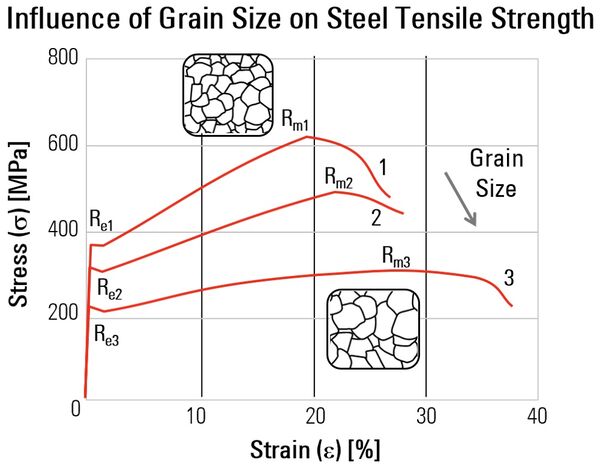
It has been well known for a long time that as the grain size increases, the alloy’s (refer to figure 1) [1]:
- tensile strength (Rm) and yield strength (Re) decrease;
- elongation at fracture (A%) increases; and
- ductile-brittle transition temperature increases.
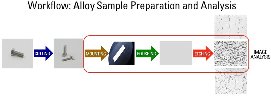
Microstructure analysis: alloy sample preparation workflow
In order to characterize the microstructure of an alloy, a sample has to be prepared from the alloy material, then ground and polished, imaged with a microscope, and finally the images are analyzed. Figure 2 shows a diagram illustrating the typical workflow for sample preparation and microstructural analysis.
Techniques for microstructure analysis
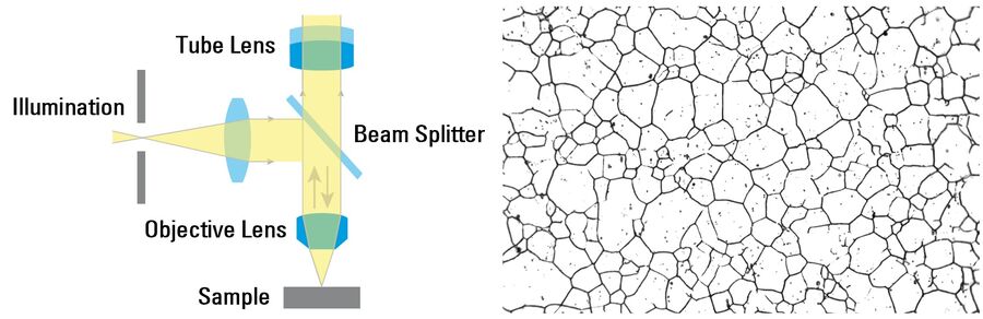
Different types of experimental techniques are used to investigate the microstructure of alloys. For more than 100 years, optical microscopy, using incident brightfield, darkfield, differential interference contrast (DIC), and polarized light illumination along with color etching, has been the most common method. At the present time, computer automated microscopes and image analysis systems provide a rapid and accurate way to evaluate such alloys.
The setup and analytical capabilities of the imaging software used has a very important effect on the accuracy, reliability, reproducibility, and efficiency of:
- image capture and analysis;
- grain size and microstructure evaluation; and
- report generation from the results.
LAS/LAS X Grain Expert software
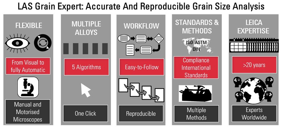
A Leica microscope using the LAS Grain Expert software offers a practical solution for accurate and reproducible grain size and microstructural analysis. Grain size can be analyzed by using automatically applied traditional methods or superior digital approaches. The analysis methods conform to various international standards. The advantages of the software are summarized in table 1 below.
LAS Grain Expert Advantages | ||||
Flexible Analysis | Analyze Multiple Alloys | Analysis Workflow | Standards & Methods | Leica Expertise |
Analysis from visual to fully automatic possible | 5 software algorithms available | Easy-to-follow guidance for using software | Fully compliant with international standards | More than 20 years experience in metallography |
Used with both manual and automated optical microscopes | Perform the measurements with just one click | Efficient analysis with reproducible results | Multiple methods for analysis available | Metallography experts available worldwide |
Table 1: Advantages of the LAS Grain Expert software from Leica Microsystems for grain size analysis.
Grain analysis methods with optical microscopy
Incident illumination contrast methods
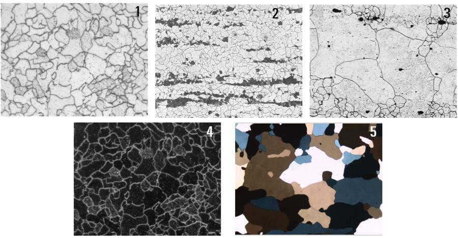
To image an alloy sample, which is opaque and cannot transmit light, optical microscopes exploit incident illumination methods. For better contrast of specific alloy microstructural components, certain contrast techniques are used [2,3]:
- brightfield;
- darkfield;
- differential interference contrast (DIC); and
- polarized light.
These incident illumination contrast methods are further explained below and in more detail in references 2 and 3.
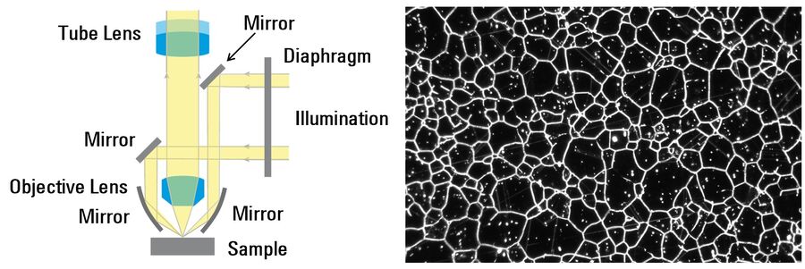
Brightfield
Advantage: Brightly illuminates uniformly the entire part of the alloy sample under observation.
Disadvantage: For reflective alloy samples, some features, such as grain boundaries, may be “drowned out” by the bright illumination and not easily visible in the image.
An image of steel alloy recorded with a compound microscope using brightfield illumination is shown in Figure 3 below.
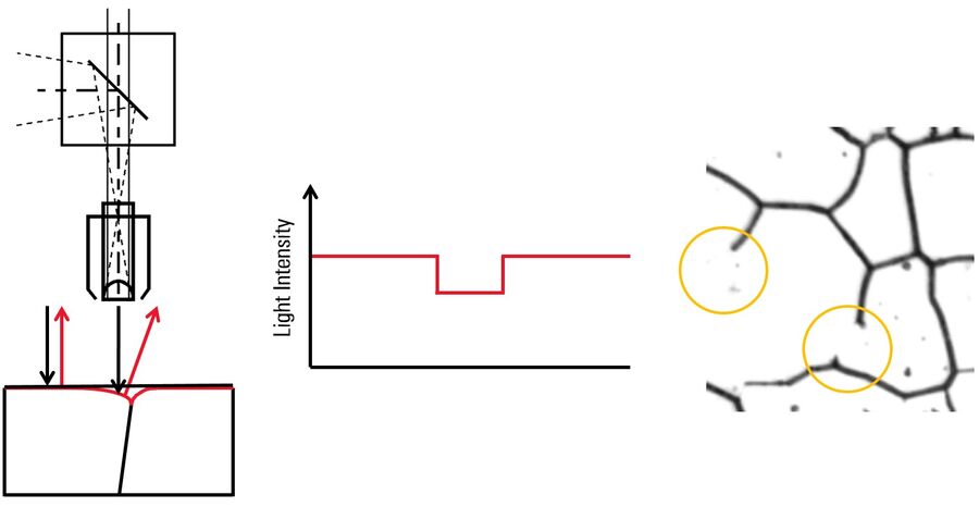
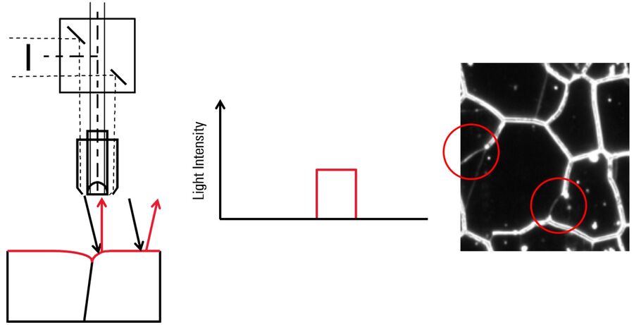
Darkfield
Advantage: Illuminates small features on flat areas of the alloy sample which cannot be seen easily with brightfield, such as cracks, pores, etched grain boundaries, fine protrusions, etc.
Disadvantage: Only for observing features which deviate from a flat alloy sample area, as the alloy background will appear dark in the image.
Figure 4 shows an image of a steel alloy taken with a compound microscope using darkfield illumination.
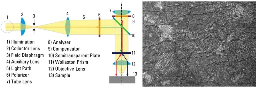
Differential interference contrast (DIC)
Advantage: Illuminates small height differences on the alloy sample enhancing the texture and feature contrast.
Disadvantage: More challenging to use and costly to implement.
An image of steel alloy recorded using a compound microscope and DIC illumination is shown in Figure 5 below.
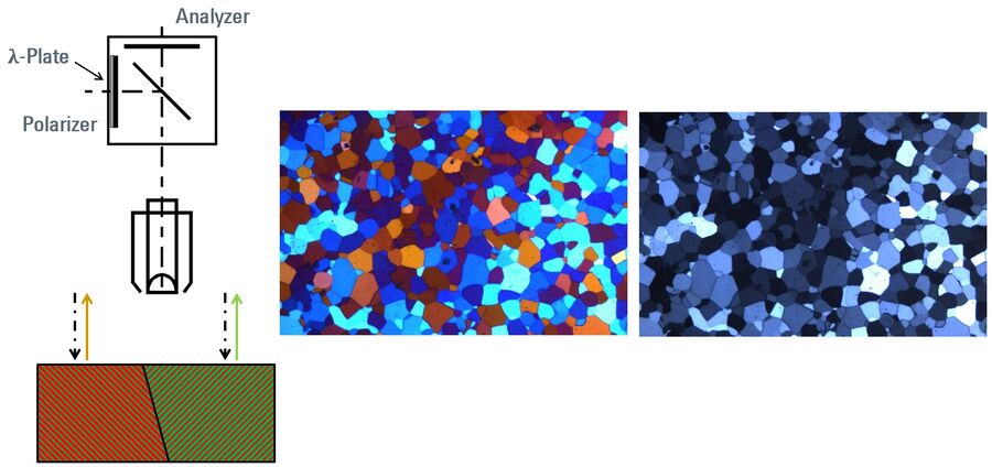
Polarized light
Advantage: Helps to enhance the observation of grains (crystallographic regions) in certain alloys. The grains often reflect specific colors (wavelengths) of the polarized light, depending on their crystallographic orientation, giving rise to color contrast.
Disadvantage: Only applicable to alloys that do not crystallize with a cubic lattice structure, such as, face centered cubic (fcc) or body centered cubic (bcc). This fact unfortunately excludes many of the major commercial alloys (steel, copper, and aluminum), however, color etching can be exploited to remedy this problem [2,3].
Figure 6 shows a tint etched aluminum alloy imaged with a compound microscope using polarized light illumination.
Etching alloys for grain contrast
In order to better see an alloy’s grains and microstructure, during sample preparation often etching with acids, bases, or electrolytic solutions is performed. During the etching, specific components of the alloy microstructure are attacked, such as the grain boundaries or phases within the grain areas. The etched alloy is then imaged normally using brightfield or darkfield illumination [2,3]. More about brightfield and darkfield imaging of etched alloys is explained below. Color or tint etching is also possible to contrast the alloy grains and microstructure [2,3]. For more details about etching of alloys, refer to references 2 and 3.
Brightfield illumination
An image of etched steel alloy recorded using a compound microscope and brightfield illumination is shown in Figure 7.
Darkfield illumination
Figure 8 shows etched steel alloy imaged with a compound microscope using darkfield illumination.
Standard grain size analysis methods
The international standard methods for grain size analysis are summarized in table 2 below.
Grain Microstructure Analysis | International Standard Method | |
Determining average grain size | ||
Determining average grain size using semiautomatic and automatic image analysis |
| |
Characterization of duplex grain sizes | ||
Estimating largest grain size: ALA (As-Large-As) grain size |
| |
Table 2: International standard methods for determining grain size in alloys.
Determining the average grain size: grain size number
The average grain size of an alloy is generally expressed in terms of the grain size number, G, as indicated in the standard ASTM E112 - 13 [4]. The value of G ranges from 00 to 14 where 00 corresponds to an average grain diameter of 0.508 mm and area of 0.2581 mm2 and 14 a diameter of 2.8 µm and area of 7.9 µm2. To evaluate the grain size number of an alloy, common methods include the intercept, planimetric, and comparison procedures described in the standards ISO 643:2012 and ASTM E112 - 13 [4,5].
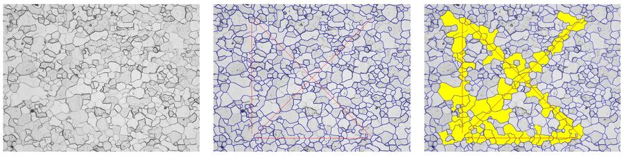
Intercept procedure
A geometric pattern with intercept lines is drawn on a microscopic image of an alloy [4,5]. The mean lineal intercept length, l, is calculated from the number of (refer to figure 9):
- grains intercepted by a test line (PL) or
- grain boundary intersections by a test line per unit length of the test line (NL).
Once PL and NL are counted and known, then the intercept length:
l = 1/PL = 1/NL
is used to determine the grain size number, G, with the formula:
G = -6.6457*log[l] – 3.298.
The greater the number of intercepts or intersections, the greater the precision of G. Generally, the intercept method is fast and delivers good accuracy.
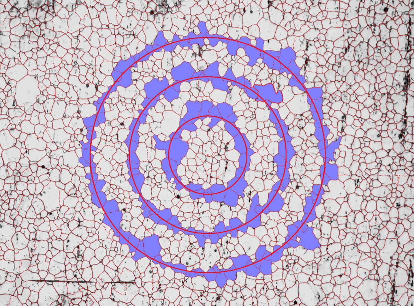
Planimetric procedure
With this method, the number of grains within a defined circular area are counted [4,5]. The number of grains per unit area, NA, is used to determine G (grain size number). The value of NA is calculated with:
NA = (M2/A)*(ninside+[nintercepted/2])
where M is the magnification, A is the circular area, ninside is the number of grains falling completely within the circle, and nintercepted is the number of grains intercepted by the circle’s perimeter (refer to figure 10). Then G can be calculated from the equation:
G = -3.322*log[NA] – 2.954.
The greater the number of grains counted, the greater the precision of G. In general, results from the planimetric method are very reproducible and precise.
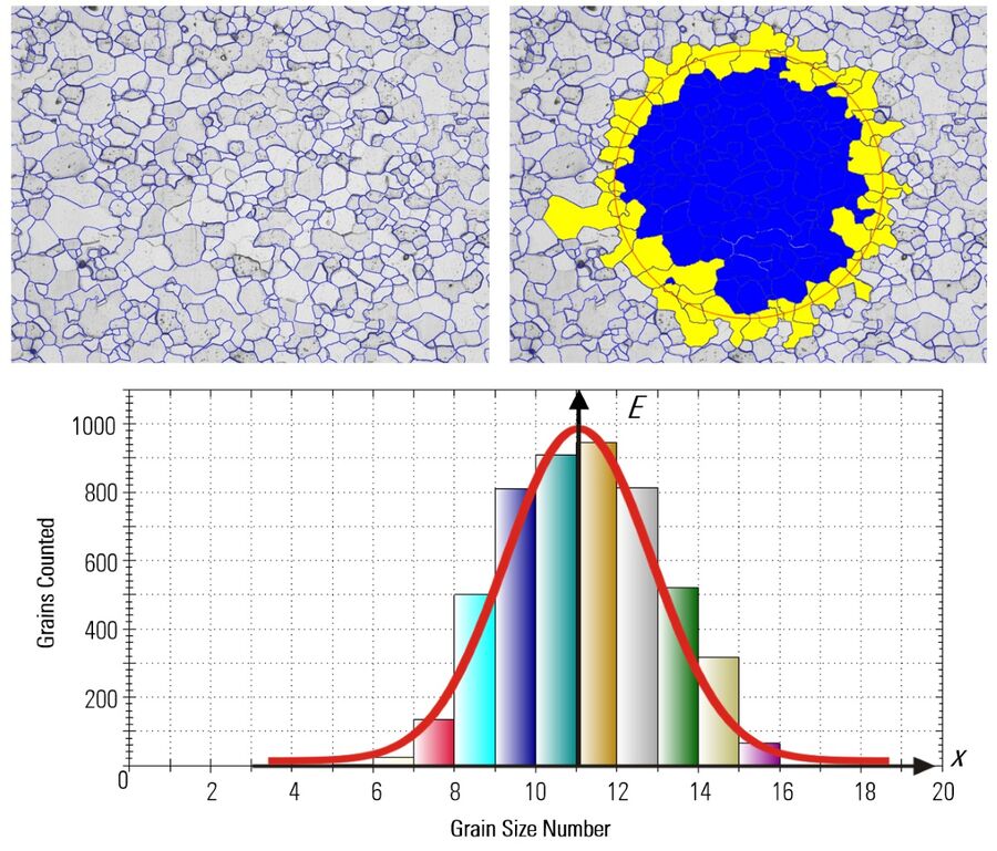
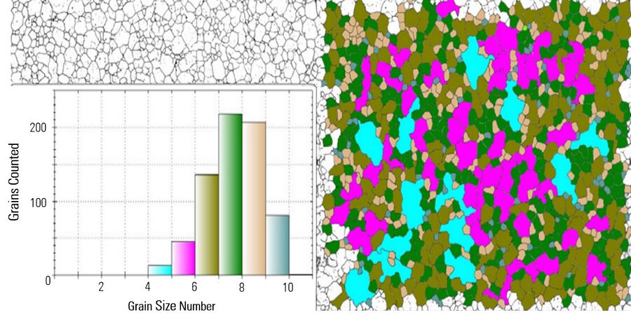
Figure 10: Example of the planimetric method used to measure the grain size of a steel alloy. A raw image (top left) was acquired with a Leica microscope using the LAS Grain Expert software. The image data was processed [top right] with the planimetric approach to determine the values of A, ninside, nintercepted, NA, and G. Blue indicates grains completely within the defined circular area and yellow those intercepted by the perimeter. Example of a histogram (bottom), with a mean G value of approximately 11, showing the grain size number distribution obtained with the planimetric analysis.
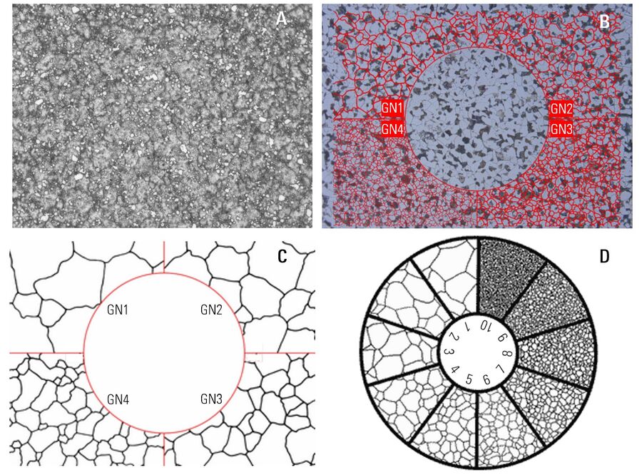
Comparison procedure
This method does not require counting, but rather comparing of the grain structure to a series of reference images recorded at 100x magnification, either in the form of a wall chart, clear overlays, or on a microscope eyepiece reticle (refer to figure 11) [4,5]. The method is fast, but the grain size values are much less accurate than those calculated from the intercept or planimetric approaches above.
Determining average grain size with semiautomatic and automatic analysis
To evaluate the average grain size of an alloy with semiautomatic or automatic analysis (software), methods are described in the standard ASTM E1382 - 97(2015) [6]. The mean grain size and the grain size distribution are evaluated using the intercept or planimetric methods discussed above. The precision and accuracy of the results depend on the quality of the alloy sample, sample preparation, imaging system, and image analysis software. An example done with the planimetric method is shown in figure 12.
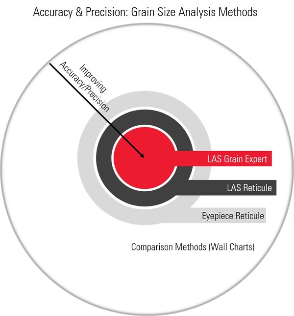
Accuracy of grain size: Automated, semiautomated, or manual analysis
In general, results obtained with automated analysis are more accurate, precise, and acquired more rapidly than either semiautomated analysis or comparison via eyepiece reticule overlays or wall charts. Likewise, semiautomated analysis is more accurate and rapid than manual analysis with eyepiece reticule overlays. An example of automated analysis would be a Leica microscope using the LAS Grain Expert software which is capable of performing both the planimetric and intercept procedures. A semiautomated analysis is possible with the LAS Reticule software via digital reticule overlays displayed on a monitor. A comparison of the accuracy of the methods is shown in figure 13.
Characterizing duplex grain size
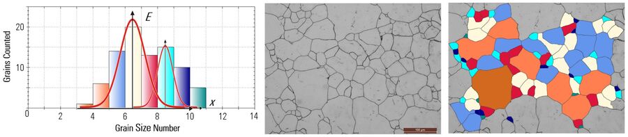
Duplex grain size can occur in some alloys after thermomechanical processing. A duplex grain size in alloys can include systematic grain size variation, necklace and banded structures, as well as germinative grain growth in areas where there is critical strain. To better understand the alloy’s mechanical properties, it can be important to characterize duplex grain size. The standards ISO 14250:2000 and ASTM E1181 - 02(2015) describe the guidelines for determining if there is a duplex grain size in an alloy [7,8]. They also clarify how to classify the duplex grain sizes into 1 of 2 distinct classes and specific types within those classes. Figure 14 shows an example of a steel alloy with a duplex grain size.
Determining largest grain size: ALA (As-Large-As) grain size analysis
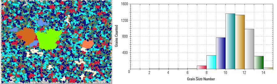
Unusually large grains in alloys correlate with anomalous behavior concerning crack initiation and propagation, as well as material fatigue. For this reason, the ALA grain size was created for alloy characterization. The standard ASTM E930 - 99(2015) explains the methods used to determine ALA grain size [9], i.e. to measure the size of unusually large grains present in an alloy with an apparent uniform distribution of grain sizes. Refer to figure 15 and table 3 for an example of ALA analysis.
Statistical Data ALA Analysis Steel | |||
Bin / Interval | Grain Size Number (G) | Count | |
G Upper Limit | Lower Limit | Upper Limit | Number of Grains |
1 | 0.0 | 1.0 | 0 |
2 | 1.0 | 2.0 | 0 |
3 | 2.0 | 3.0 | 1 |
4 | 3.0 | 4.0 | 1 |
5 | 4.0 | 5.0 | 1 |
6 | 5.0 | 6.0 | 3 |
7 | 6.0 | 7.0 | 12 |
8 | 7.0 | 8.0 | 79 |
9 | 8.0 | 9.0 | 333 |
10 | 9.0 | 10.0 | 772 |
11 | 10.0 | 11.0 | 1362 |
12 | 12.0 | 12.0 | 1330 |
13 | 12.0 | 13.0 | 980 |
14 | 13.0 | 14.0 | 316 |
15 | 14.0 | 15.0 | 29 |
Table 3: Data from grain size measurements done on steel using ALA analysis.
Difficult cases for grain size analysis
Difficulties can arise during alloy grain size analysis due to:
- artifacts from sample preparation;
- poorly revealed grain boundaries;
- over-etching of sample;
- tangled microstructure;
- twinning
To obtain accurate results with LAS Grain Expert, it is important to choose a good quality alloy sample and sample preparation method [6]. If sample preparation does not deliver good results or the microstructure deviates from what is normally expected, then the user can apply the LAS Reticule solution to have an estimate of the mean grain size with a precision of ± 0.5 G.
Practical solution: Leica microscope with LAS Grain Expert Software
Algorithms to detect grain boundaries
There are 5 different algorithms used in the LAS Grain Expert software to detect grain boundaries:
- single phase;
- dual-phase;
- duplex condition;
- dark field;
- polarized light.
Users select the processed image (see figure 16) which best resembles their actual alloy sample.
Detailed grain size analysis
The LAS Grain Expert software is able to express the average grain size in terms of G (grain size number) and calculate the:
- grain size number distribution, standard deviation, and other statistical values;
- mean grain area;
- maximum and minimum grain size;
- confidence level (p value);
- relative accuracy of the results.
Refer to table 4 and figure 17 for an example of analysis with the LAS Grain Expert software.
Statistical Data LAS Grain Expert Analysis Steel | |||
Bin / Interval | Grain Size Number (G) | Count | |
G Upper Limit | Lower Limit | Upper Limit | Number of Grains |
1 | 0.0 | 1.0 | 0 |
2 | 1.0 | 2.0 | 0 |
3 | 2.0 | 3.0 | 0 |
4 | 3.0 | 4.0 | 0 |
5 | 4.0 | 5.0 | 2 |
6 | 5.0 | 6.0 | 7 |
7 | 6.0 | 7.0 | 19 |
8 | 7.0 | 8.0 | 38 |
9 | 8.0 | 9.0 | 89 |
10 | 9.0 | 10.0 | 102 |
11 | 10.0 | 11.0 | 120 |
12 | 12.0 | 12.0 | 68 |
13 | 12.0 | 13.0 | 72 |
14 | 13.0 | 14.0 | 42 |
15 | 14.0 | 15.0 | 21 |
16 | 15.0 | 16.0 | 13 |
Table 4: Data from analysis of grain sizes in steel made with the LAS Grain Expert software.
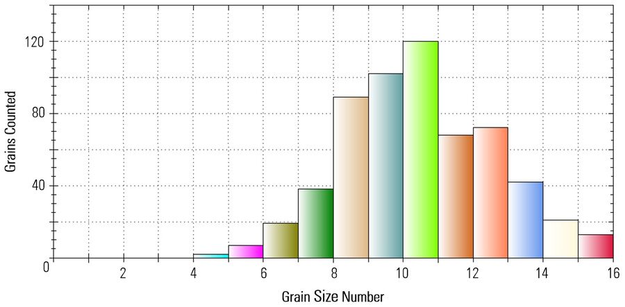
Figure 17: Histogram showing the grain size number distribution for steel alloy. Data was obtained from analysis done with the LAS Grain Expert software. The mean grain size number = 10.76, standard deviation (σ) = 1.63, mean grain area = 134.55 μm2, and mean grain diameter = 11.23 μm.
Summary
In this report, the importance of grain size analysis for alloys used in the automotive and transportation industries has been reviewed. In addition, a precise, practical solution for its analysis using automated, digital microscopy methods have been discussed.
A Leica microscope using the LAS Grain Expert software provides an accurate, reliable, and efficient method for obtaining grain size results and evaluating the data. It also makes batch processing and report generation as easy as one click. Refer to figure 18 for an overview of the advantages in terms of using the LAS Grain Expert software from Leica Microsystems.
Further Reading
- M. Cavallini, V. Di Cocco, F. Iacoviello, Materiali Metallici, Terza Edizione, ISBN 978-88-909748-0-9, Luglio 2014.
- Dionis Diez, Metallography – an Introduction: How to Reveal Microstructural Features of Metals and Alloys, Science Lab, Leica Microsystems.
- Ursula Christian, Norbert Jost, Metallography with Color and Contrast: The Possibilities of Microstructural Contrasting, Science Lab, Leica Microsystems.
- ASTM E112 – 13: Standard Test Methods for Determining Average, Grain Size, ASTM International.
- ISO 643:2012: Steels -- Micrographic determination of the apparent grain size, International Organization for Standardization.
- ASTM E1382-97(2015): Standard Test Methods for Determining Average Grain Size Using Semiautomatic and Automatic Image Analysis, ASTM International.
- ISO 14250:2000: Steel -- Metallographic characterization of duplex grain size and distributions, International Organization for Standardization.
- ASTM E1181-02(2015): Standard Test Methods for Characterizing Duplex Grain Sizes, ASTM International.
- ASTM E930 - 99(2015): Standard Test Methods for Estimating the Largest Grain Observed in a Metallographic Section (ALA Grain Size), ASTM International.
Related Articles
-

Unlocking Insights in Complex and Dense Neuron Images Guided by AI
The latest advancement in Aivia AI image analysis software provides improved soma detection,…
Jun 16, 2023Read article -

AI Microscopy Enables the Efficient Detection of Rare Events
Localization and selective imaging of rare events is key for the investigation of many processes in…
Jun 06, 2023Read article -

Accurately Analyze Fluorescent Widefield Images
The specificity of fluorescence microscopy allows researchers to accurately observe and analyze…
Jan 17, 2022Read article