The Power of Pairing Adaptive Deconvolution with Computational Clearing

Since the invention of the microscope in 1595 [1], the discovery of fluorescence and the first description of light microscopy in visualizing stained samples in the 1850’s [1], widefield (WF) fluorescence microscopy has become a widely used imaging technique that has benefited the disciplines of engineering and science. Our scientific curiosity continues to drive the development of microscopy forward, with the goal to see and resolve more structural detail. However, due to the wave nature of light and the diffraction of light by optical elements, image resolution is limited by the diffraction spot known as the diffraction limit. In WF fluorescence microscopy both the contrast and resolution of a captured image is reduced by multiple sources including: light collected from adjacent planes, scattered light, and camera sensor noise, all of which increase image haze/blur (background noise). Additional losses in image resolution and contrast can be tied to the systems optical response function commonly known as the point spread function (PSF). The PSF describes what an idealized point source would look like when imaged at the detector plane and operates as a low pass frequency filter that filters out the high spatial frequency content in the image, Figure 1.
Mathematically, image formation (i) can be represented as a convolution (*) between the observed object (o) and the PSF (h) with added noise (Poisson and/or Gaussian - ε ) as described by 

To minimize the effects of decreased image contrast and resolution by the PSF, image restoration techniques such a deconvolution are often used to restore and enhance the detail that is lost in the image.

Deconvolution is a computational method used to restore the image of the object that is corrupted by the PSF along with sources of noise. Given the acquired image i, the observed object o, and knowledge of the PSF (theoretically or experimentally determined) the observed object in Eq 1. can be restored through the process of deconvolution. To perform deconvolution, the object and the PSF are transformed into the frequency domain by the Fourier transform as presented in Eq 2:

For computational reasons, deconvolution is performed in the frequency domain, and Eq 1. can be re-written as shown in Eq 3. and solved for O:

where F, F–1, O, H, and £ are the Fourier transform, the inverse Fourier transform, the Fourier transformed observed object, the Fourier transformed PSF (known as the optical transfer function; OTF) and the Fourier transformed noise. However, as H approaches zero (at the edges of the PSF), both the left-most term and the noise term in Eq 3. become increasingly large, amplifying noise and creating artifacts. To limit the amount of amplified noise, the PSF can be truncated, but this will result in the loss of image detail.

Several deconvolution algorithms have been proposed [2-8] to address the above image restoration issues. For instance, the Richardson Lucy (RL) algorithm based on a Bayesian iterative approach is formulated using image statistics described by a Poisson or Gaussian noise process. By minimizing the negative log of the probability [2,3], the RL equation for deconvolution for Poisson and Gaussian noise processes are, Eq 4:

for Poisson [2,3]​​​​​​​ and

for Gaussian [10] Eq 4 where i, and o have been previously defined, and h⁺ is the flipped PSF. However, similar to Eq 3. the RL deconvolution method is susceptible to amplified noise, resulting in a deconvolution that is dominated by noise [2,3], Figure 2. Partial treatment to limit amplified image noise is to either terminate the convergence early, or to carefully select a value for o_k that is pre-blurred with a low pass frequency filter (ex. Gaussian filter) [2,3]​​​​​​​. More recently, new deconvolution methods have been proposed that use a regularization term that can be added to the algorithm that constrains the deconvolution. Such regularization techniques include methods like Tikhonov-Miller, Total-Variation, and Good’s roughness [2,4-9]​​​​​​​​​​​​​​. The purpose of these regularization terms is to penalize the deconvolution to limit image noise and artifact generation with the goal to preserve image detail.

The method used by Leica Microsystems is an accelerated adaptive RL approach that is regularized and constrained using Good’s roughness [11]​​​​​​​. Using a Bayesian statistic approach with a Gaussian noise process, the function to minimize for deconvolution is:

where γ is the regularization term, ∇ is the differentiation operator, and h is the Gibson-Lanni PSF. In Eq 5., the regularization term, γ, is dependent on the local signal-to-noise ratio (SNR) and is a function of adaptive SNR (x, y) coefficients created over the entire image, Figure 3. Together, γ∫1[∇o]2, acts to penalize the deconvolution, and the regularization term scales non-linear with SNR (x, y) as:

with SNRmax defined as a predetermined maximum SNR value, and γmax is the maximum predefined regularization. The result is the adaptive regularization of Eq 5., yielding greater penalization to the deconvolution for regions having lower SNRs in contrast to regions with higher SNRs. This yields a deconvolution process that is properly regularized over the entire image avoiding image artifacts and the amplification of noise.

Using the deconvolution algorithm offered by Leica Microsystems the user can define the number of iterations for deconvolution or use the default option to have the algorithm determine the stop criterion for convergence. The latter option is more time efficient, and removes the guesswork required by the user. Similar to Leica Microsystems Instant Computational Clearing (ICC) algorithm, the described adaptive deconvolution method is included on all THUNDER imaging systems and is fully integrated into the imaging workflow [12].

How well deconvolution performs on a widefield fluorescent image is dependent on several factors including the amount of light collected from adjacent planes, the sample thickness, the degree of scattered light, and the SNR of the image. For instance, in thick specimens an appreciable amount of light scattering can occur within the sample resulting in the failure of deconvolution to produce a restored image with improved resolution and contrast. For samples that have high SNR with minimal background noise, deconvolution can yield over processed images resulting in unwanted sharp boundary transitions between image features. Therefore, the need for an imaging workflow that is adaptable for diverse sample thicknesses with varying SNRs is important.

In our previous technology brief we discussed Leica Microsystems ICC algorithm as a method to restore image contrast through the removal of background noise. This is done through the minimization of a non-quadratic cost function that estimates and subtracts the background noise from the image to improve contrast [12]​​​​​​​. To address the previously mentioned pitfalls of deconvolution, Leica Microsystems introduced a workflow that combines both computational algorithms, allowing users to perform ICC, or ICC with deconvolution. For the latter, the pairing is selectable between two different processing modalities based on the sample thickness and SNR, referred to as small and large volume computational clearance, SVCC and LVCC respectively.

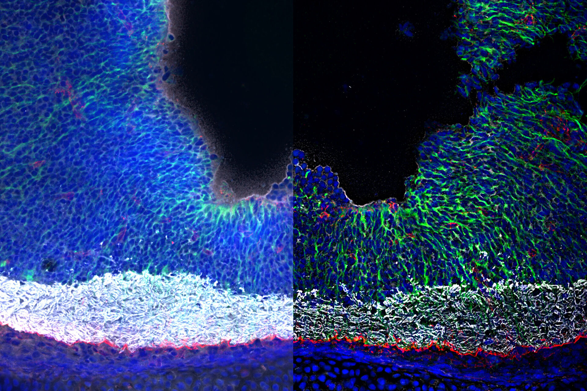
When using SVCC, the adaptive deconvolution is performed prior to THUNDER ICC. In SVCC, a theoretical PSF is used in the deconvolution with knowledge of the systems optical parameters (the type of microscope objective, the emission wavelength, the sample embedding media, etc.). The choice in using SVCC is especially important for ‘noisy’ images, Figure 4, since the adaptive deconvolution will improve the SNR prior to the automatic removal of the unwanted background via ICC, Figure 4C. In LVCC, ICC is performed prior to deconvolution and uses a PSF that is influenced by the parameters of ICC. LVCC is ideally suited for samples that have higher SNRs and more background noise contributions that are common in thick samples, Figure 5. By performing ICC prior to deconvolution, the contrast of the spatial features is enhanced, Figure 5C, allowing for a more precise treatment of the remaining signal through deconvolution.

For both SVCC and LVCC, the strength of ICC is user adjustable. The strength parameter (s) scales the amount of estimated background intensity (Ibackground) that is subtracted from the image (I) resulting in the final image (I'):

Together the strength parameter, SVCC, and LVCC allow the user to fine tune the computational algorithm to their sample for the best treatment of their data. As with ICC, both SVCC and LVCC can be applied during image acquisition or post-acquisition, with the raw data always being preserved. This means that the user can directly compare the raw data to the processed data for further quantification. The topic of quantification will be discussed in our next upcoming technology brief.

We would like to thank Kai Walter (Software engineer), Louise Bertrand (Product Performance Manager Widefield) and Jan Schumacher (Advanced Workflow Specialist) for reading and providing their comments on this technical brief.

1. Heinrichs, A. (2009, October 1). (1858, 1871) First histological stain, Synthesis of fluorescein. Retrieved November 09, 2020
2. Sibarita, J. (2005). Deconvolution Microscopy. Microscopy Techniques Advances in Biochemical Engineering/Biotechnology, 95, 201-243. doi:10.1007/b102215
3. Dey, N., Blanc-Féraud, L., Zimmer, C., Roux, P., Kam, Z., Olivo-Marin, J., Zerubia, J. (2004). 3D Microscopy Deconvolution using Richardson-Lucy Algorithm with Total Variation Regularization.
4. Rodriguez, P.,. (2013). Total Variation Regularization Algorithms for Images Corrupted with Different Noise Models: A Review. Journal of Electrical and Computer Engineering. 2013. 10.1155/2013/217021.
5. Tao, M., Yang, J. (2009). Alternating direction algorithms for total variation deconvolution in image reconstruction. Optimization Online.
6. Roysam, B., Shrauner, J. A., Miller, M. I., (1988) Bayesian imaging using Good's roughness measure-implementation on a massively parallel processor, ICASSP-88., International Conference on Acoustics, Speech, and Signal Processing, New York, NY, USA, , pp. 932-935 vol.2, doi: 10.1109/ ICASSP.1988.196742.
7. Verveer, P., Jovin , T., (1998) Image restoration based on Good’s roughness penalty with application to fluorescence microscopy, J. Opt. Soc. Am. A 15, 1077-1083
8. Zhu, M., (2008). Fast Numerical Algorithms for Total Variation Based Image Restoration, [Unpublished Ph.D. dissertation] University of California, Los Angeles.
9. Good, I., & Gaskins, R. (1971). Nonparametric Roughness Penalties for Probability Densities. Biometrika, 58(2), 255-277. doi:10.2307/2334515
10. Oyamada, Y. (2011). Richardson-Lucy Algorithm with Gaussian noise.
11. D. Zeische, F. and Walter, K., Leica Microsystems CMS GmbH, Deconvolution Apparatus and Method Using a Local Signal-to-Noise Ratio, Germany, 18194617.9, 14.09.2018.
12. Felts, L., Kohli, V., Marr, J., Schumacher, J., Schlicker, O. (2020, October 01). An Introduction to Computational Clearing. Retrieved November 09, 2020