 dataset, showing the biochemically distinct structures of a fresh, untreated apple slice.")
SRS Sample Preparation
- The SRS signal is detected in transmitted-light mode. Therefore, as a rule of thumb, specimens should be at least semitransparent.
- Thicker or less transparent samples should be sectioned to a suitable thickness, whenever the experiment allows for it. In our experience, 10-100-micrometer-thick slices work well. Alternatively, thick samples can be investigated using CARS microscopy which can be detected in both transmitted- and incident-light (epi-illumination) modes.
- Specimens can be fresh or formalin fixed. Methanol fixation is discouraged for lipid related analysis, because this method is known to extract lipids from the specimen. When studying molecules other than lipids, the signal from the lipid content might be a problem for the signal-to-noise ratio (SNR), so for that reason methanol fixation could be beneficial.
- For fresh samples, care has to be taken during long spectroscopy scans, as it may be necessary to identify potential motion artifacts.
- Specimens can be sandwiched between a coverslip and a microscope slide. In contrast to spontaneous Raman scattering, signals from out-of-focus regions are highly suppressed by nonlinear optical signal generation. Hence, fluorescence background signals from the substrate and other components in the beam path are virtually nonexistent. Also, there are no special requirements for the substrate material. The position of the specimen in the sandwich construction should be within the working distance of both the objective and condenser (see below). Thus, ideally, the specimen should be in direct contact with the surface of the cover glass and microscope slide.
- It is preferred to mount samples in aqueous solution or buffer, e.g., sandwiched using double-sticky spacers. When necessary, samples can be embedded (typical fluorescence mounting media like Mowiol or Dako and hydrogels such as Matrigel or Agarose should work). Paraffin embedded sections can be analyzed with or without removal of the paraffin. However, we strongly recommend removing it.
- Alternatively, specimens in a glass-bottom petri dish can be imaged, e.g., with the STELLARIS 8 CRS microscope using a S1 oil condenser in a water dipping configuration.
- In many cases, even fluorescently labeled specimens can be probed by SRS without fluorescence cross-talk into the SRS channel. Therefore, it is possible to correlate fluorescence images with SRS signals. The immunity of SRS to most fluorescent signals arises from the lock-in-based detection scheme coupled with the very-much red-shifted detection band. In rare cases, when fluorescent contamination signals are present, often they can be separated from true SRS signals in a spectral analysis (fluorescence signals will have a weak spectral dependence, if any, whereas SRS signals will show pronounced spectral peaks).
SRS imaging workflow
A suitable choice of objective is crucial for CARS/SRS, as the Pump/Stokes pulses must overlap in 3D space and time to achieve optimal signal strength. Suggested objectives are:
- 10x NA=0.4 Air HC PL APO CS
- 20x NA=0.75 Water HC PL IRAPO
- 25x NA=0.95 Water HC FLUOTAR VISIR 0.17
- 40x NA=1.1 Water HC PL IRAPO CORR (Note: optimizing the position of the CORR ring for each sample may have a dramatic effect on signal strength and image quality)
Please note that for each objective the temporal overlap of the pump and probe pulses must be optimized. This delay calibration should be performed by Leica service personnel.
For SRS microscopy, it is strongly recommended to use a condenser with a numerical aperture (NA) larger than the NA of the excitation objective! If this condition is not fulfilled, spurious non-SRS signals can arise. S1 condensers (NA=0.9 air or 1.4 oil) are recommended.
For a first inspection, we suggest imaging the specimen at a vibrational frequency where the most intense signals are expected (for typical biological specimens, this will be in the CH-stretch region, e.g. at 2850 cm-1 for lipid-rich specimens or 2935 cm-1 for protein-rich ones). At this vibrational frequency, adjust the laser power and detector gain to utilize the full dynamic range of the image. Typical parameters for SRS imaging are shown in Table 1.
| Pump, Stokes Powers in Laser GUI | 150 mW (Pump), 300 mW (Stokes) at laser output; Keep 1:2 ratio. Do not exceed 150mW Pump to avoid damage to SRS detector! |
| Intensity slider | 20-40% |
| SRS detector gain | ~10% of full scale. Increase only if laser power maxed out. |
Table 1: Typical acquisition parameters for SRS microscopy.
Additional signals, such as Epi-CARS and Epi-SHG/2PF, often provide further valuable information about the specimen and can be acquired in parallel. Optimize the acquisition parameters for these channels as well.
SRS spectroscopic imaging
Before starting a spectral scan, sufficient time should be allowed for the microscope to reach a steady-state temperature and for the specimen to settle. This precaution will help avoid z-drifts during spectral scans.
To set up a spectral scan, choose the xyΛ or xyzΛ scan mode.

In the Lambda Scan Window shown in Figure 1, select the start and end points and the step size of the scan. We suggest breaking down spectral scans into two regions, the high-wavenumber region (HWR, ~3100 cm-1 to ~2800 cm-1) and the fingerprint region (FPR, ~1800 cm-1 to ~600 cm-1), because these regions differ in their signal strengths and spectral complexity.
Typical scans of the HWR will be comprised of 30-40 spectral points, have a step size of 0.5 nm, and can be acquired in one piece.
For scans of the FPR, a smaller step size of 0.4 nm is recommended to sample the narrower spectral features adequately. Scans of the entire fingerprint region can easily be comprised of 200-300 spectral points and should be broken down into several pieces. This step is recommended to retain the optimal stability of the laser parameters while tuning it. Each partial scan can either be set up manually or as a sequence of xyΛ jobs in Live Data Mode. The separate image series from partial scans can be merged later with the processing tool and analyzed together.
FPR signals in biological specimens are typically 5-10x weaker than HWR signals. This often requires an increase in laser power (typically ~50% higher than for HWR scans), an increase in SRS detector gain (typically 2x-3x higher than for FPR scans), and, depending on the desired signal-to-noise ratio (SNR), possibly further signal enhancements through line/frame averaging or accumulation.
As FPR spectra can be quite complex, care should be taken that signals will not be saturated at any spectral point from any structure of interest in the specimen. If the vibrational frequencies of most intense signals is known beforehand, the acquisition settings for the FPR scans should be optimized for these frequencies. If it is not known, then typical candidate frequencies would be the total lipid signal at ~1445 cm-1 or, in some cases, the unsaturated lipid signal at ~1655 cm-1.
Below in Figure 2 the workflow is illustrated with an example of a spectral analysis of fingerprint signals from a freshly-cut apple slice, looking at the peel and outer regions of the fruit’s flesh.

Analysis of spectral data:
SRS spectra are mathematically identical to spontaneous Raman spectra and, hence, lend themselves to the same types of quantitative analysis procedures that have been developed for spontaneous Raman spectroscopy. In practice, SRS spectra are probably even more easily interpreted, because there is virtually no fluorescence background contamination and, as a result, there is no requirement for data preprocessing steps like background subtraction procedures.
A) User-Defined Spectral Analysis
A user-defined spectral analysis begins by selecting regions of interest (ROIs) and displaying their spectra in LAS X, as shown in Figure 3: Under the “Quantify” Tab, choose “Stack Profile”, Dimension: Λ. Note, the x-axis of the spectra can be displayed in terms of the vibrational frequency, also called Raman shift (cm-1 units), or in terms of the pump laser wavelength λPump (nm units). The wavelength units can be converted to vibrational frequencies using the formula:
v [cm-1] = 107 (1/λPump[nm]-1/λStokes[nm])
The Stokes laser wavelength λStokes is fixed and its precise value can be read off from the laser line display. Spectra can be exported via a right mouse click on the spectra and selecting “Export” to “Excel” format. Also, note that the image ROIs can be saved as well for future use in LAS X (right click on the image when displayed in the “Quantify” tab → “Save ROIs”).
 of the image.")
B) Spectral Dye Separation
An alternative fast and intuitive method of discriminating sample substructures, based on their spectral signatures, is the “Spectral Dye Separation” feature, built-into the LAS X software. This is illustrated in Figure 4 below.
Under the “Process” tab, select “Dye Separation” → “Spectral Dye Separation”. Again, ROIs can be selected and corresponding spectra can be saved/exported into the dye database. A desired number of these spectra can then be selected as the basis for separation.
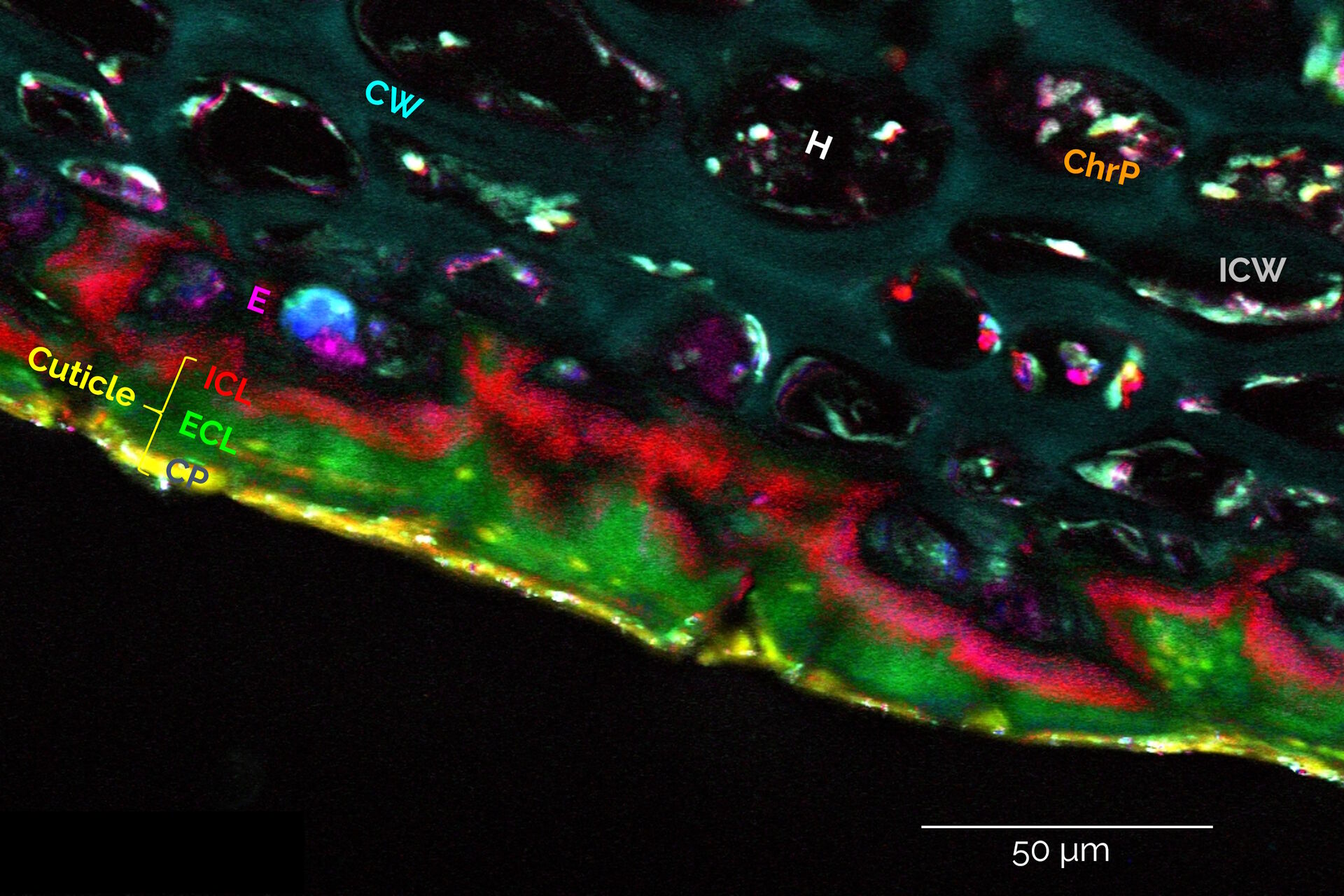
 Illustration of the Spectral Dye Separation user interface. (B) Example result showing 8-color separation of a hyperspectral data set from an apple slice. (C) Overlay of the 8 colors.")
As Figure 4 demonstrates, this method is suitable to discriminate and visualize at least 8 biochemically distinct substructures in an apple specimen (same hyperspectral dataset as shown in Figure 1), revealing different cuticular layers of the apple peel with highly distinct lipid compositions, the carbohydrate-rich flesh of the fruit, various pigments containing carotenoids, and other compartments containing high concentrations of polyphenols.
C) Automatic Dye Separation
If only a few images at distinct vibrational frequencies are acquired, instead of a full hyperspectral image stack, then the “Automatic Dye Separation” can be used to display distinct biological components of the sample. Figure 5 shows the separation of a 6-color SRS image stack of a mouse brain sliced into three components representing lipid-rich white matter and myelinated axons (shown in red), protein-rich gray matter (green), and neuronal cell nuclei (blue).

, unsaturated lipids (magenta, 3050 cm-1), collagen (SHG, cyan). Sample courtesy of R. Rudolf, J Klicks, Hochschule Mannheim")