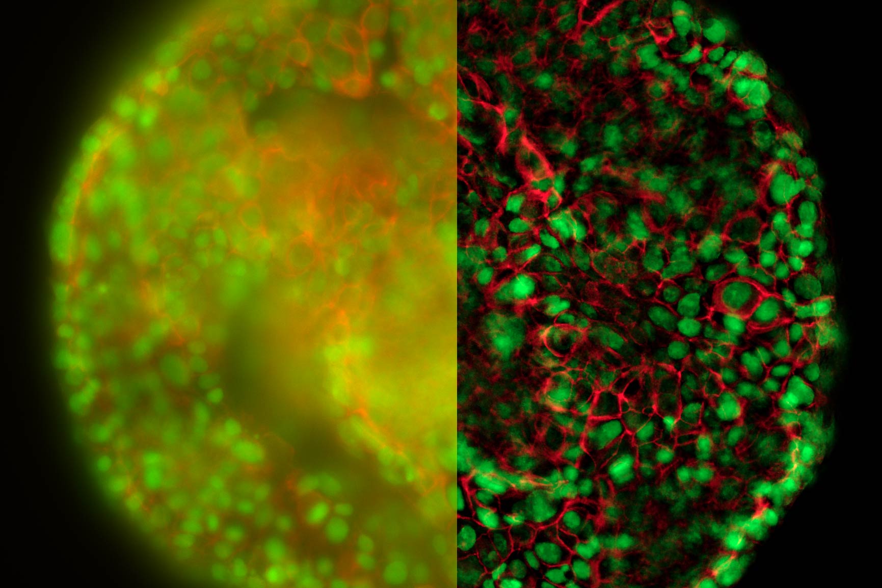
 and YOYO 1 iodide (Nucleus).")
Introduction
Methods to reduce or remove background (BG) signal
Depending on the way in which the BG caused by a out-of-focus-signal is handled, we distinguish between exclusive and inclusive methods.
Inclusive methods, such as widefield (WF) deconvolution microscopy, take the distribution of light in the whole volume into account and reassign recorded photons from the BG to their origins, thereby increasing the SNR of the recorded volumes. This reassignment can be done, because the distribution of light originating from a single point is described by the Point Spread Function (PSF). Inclusive methods reach their limits as more and more light from out-of-focus layers is combined with the light from the in-focus-region. Effects which distort the PSF, such as light scattering, increase the BG, making restoration with inclusive methods more difficult. Unfortunately, scattering is unavoidable in biological specimens. Because inclusive methods, according to their definition, use all signals detected in the image, they also process signal components from out-of-focus layers that should not contribute to the final result.
Exclusive methods are based on the principle of separating out the unwanted BG and subtracting it from the image, so only the signal from the in-focus layer remains. Camera-based systems utilize hardware to prevent the acquisition of out-of-focus light (e.g. spinning disk systems or selective plane illumination) or a combination of software and hardware to remove BG components (grid projecting systems). Grid projecting systems need multiple images to be acquired, which can lead to motion artefacts when recording fast moving samples. In addition, they work only up to a limited depth, as a sharp image of the grid needs to be detected by the camera. The gold standard in removing out-of-focus BG are pinhole-based scanning systems. The pinhole of a confocal system excludes light from out-of-focus layers, so only light from the in-focus layer reaches the detector. THUNDER Imagers use Computational Clearing as exclusive method to remove the BG with a single recorded image in real time. It therefore overcomes the disadvantages when imaging life samples as mentioned above.
Computational Clearing (CC)
Computational Clearing is the core technology in THUNDER Imagers. It detects and removes the out-of-focus BG for each image, making the signal of interest directly accessible. At the same time, in the in-focus area, edges, and intensity of the specimen features remain. When recording an image with a camera-based fluorescence microscope the “unwanted” BG adds to the “wanted” signal of the in-focus structures and both is always recorded. For best results, the aim is to reduce the BG as much as possible. To exclude unwanted BG from an image, it is critical to find key criteria necessary to accurately separate the BG from the wanted signal. Generally, BG shows a characteristic behavior in recorded images which is independent of its origin. Hence, just from its appearance in an image, it is not discernable where the BG comes from. Specifically in biological samples, the BG is usually not constant. It is quite variable over the field of view (FOV). Computational Clearing takes this automatically into account to make the in-focus signal immediately accessible.

Figure 1: Illustration of the in focus and out of focus PSF: The PSF of widefield images (center) can effectively be described by the two PSF components in focus (left) and out of focus (right). The background estimation takes advantage of the fact, that the structural length scale , S[ ̂ Iout] of the out of focus signal is larger than the corresponding structural length scale, r0, as given by the width of the in-focus signal.
How to separate out of focus from in focus signal?
Images acquired with a widefield microscope can be decomposed into two components: in-focus and BG signals. BG is mainly arising from out-of- focus signals. Thus, a widefield image, I(r), can approximately be given by:

Where psfof/if(r) and f(r) are the effective point spread functions of the in-focus (if) and out-of-focus (of) contributions and the fluorophore distribution, respectively. Because the out-of-focus PSF is much wider than the in-focus one, these two contributions in Eq. (1) can be clearly separated by length-scale-discriminating algorithms, such as, wavelet transforms. We developed an iterative algorithm to separate these two contributions. It calculates the following minimization for each iteration:

Here S[ ̂Iout] represents the structural length scale of the estimated out of focus contribution Iout. The structural length scale r0 Eq. (2) is calculated based on the optical parameters of the system and can be adapted. In the LAS X software, it is called “feature” scale.
Using this approach, only the BG is removed. Both the signal and the noise from the in-focus sample area of interest are kept. Because the noise from the in-focus area remains, the edges of in-focus features in the images are visible, therefore maintaining the spatial relations between the sample features with respect to their feature scale. The relative intensities of the features are still conserved, despite the varying nature of BG typical in life science samples.
Unlike traditional inclusive methods, the image that is revealed using Computational Clearing is not generated, but just “unmasked” from the background signals in the sample.

Information extraction: Adding Adaptive Deconvolution
Computational Clearing removes the BG, clearly revealing focal planes deep in the sample. Computational Clearing, as an exclusive method, actually becomes even more powerful when used in combination with an inclusive method.
THUNDER Imagers offer three modes to choose from:
- Instant Computational Clearing (ICC),
- Small Volume Computational Clearing (SVCC) and
- Large Volume Computational Clearing (LVCC).
Instant Computational Clearing (ICC) is a synonym of the exclusive Computational Clearing method as it was first introduced at the beginning of this technology note. SVCC and LVCC are combinations of exclusive Computational Clearing and an inclusive decision-mask- based 3D deconvolution dedicated to either thin samples (SVCC) or thick samples (LVCC). The adaptive image information extraction of the inclusive methods follows a concept that evolved from LIGHTNING, Leica Microsystem’s adaptive deconvolution method, originally developed for confocal microscopy.
LIGHTNING uses a decision mask as a base reference to calculate an appropriate set of parameters for each voxel of an image. In combination with a widefield PSF, the functionality inherent to LIGHTNING of a fully automated adaptive deconvolution process can be transferred to widefield detection.
Experimental evidence
In this section, experimental data is shown to demonstrate:
- How the data generated with THUNDER Imagers is quantifiable;
- How Computational Clearing allows imaging deeper within a sample;
- The improvement in image resolution attained with THUNDER Imagers.
Quantifying Widefield Data with Computational Clearing I
InSpeck beads are microsphere standards that generate a series of well- defined fluorescent intensity levels for constructing calibration curves and evaluating sample brightness. In this short experiment, an equal volume of same-size fluorescent and non-fluorescent beads were mixed together. The fluorescent beads had different relative intensities, i.e., 100%, 35%, 14%, 3.7%, 1%, and 0.3%.
InSpeck beads were deposited onto a cover slip and 156 positions were imaged using a 20x low NA objective (Figure 3, single z-position). Three channels were recorded (Figure 3 from left to right): bright field (BF),
phase contrast (PH) and fluorescence (FLUO). The FLUO intensity was adjusted to avoid saturation of the camera sensor from bright objects. To correct for potential inhomogeneous illumination, the central area of the
FOV was used. No further flat-field correction was performed. The FLUO images were post-processed with Instant Computational Clearing (ICC) using a feature scale of 2500 nm which corresponds to the bead size.


indicate the relative intensities of the underlying bead population. Computational-cleared data scale set to a max of 1,000 counts: 3,620 counts are in the first bin (zero to 0.1%) representing the non-fluorescent beads.
Beads were found by simple thresholding of a PH image. To correct for falsely detected beads, only round objects (≥ 0.99 roundness) of a certain size (68 to 76 pixels) were accepted. This mask was used to get the mean intensities of the raw fluorescent and the ICC processed channels. There was no exclusion of intensity outliers. To get relative values, the raw and processed intensities of all accepted beads were divided by the median intensity of their largest intensity population (usually the 100% relative-intensity fluorescent beads). In figure 4 (right), the black lines show that, following Computational Clearing, the intensities still appear around the expected values.
Conclusion: Computational Clearing allows the true fluorescent dynamics of the beads to be distinguished, even for the weakest-signal population which is not observable in the raw data. Quantification of emission intensities is easily done when using Computational Clearing. However, for such kinds of experiments, good practices for quantitative fluorescence microscopy need to be followed very closely.
Quantifying Widefield Data with Computational Clearing II
The following experiment shows how ICC deals with massive differences and heterogeneity in BG. A green-fluorescent-bead population of varying intensities was prepared and dispersed onto a cover slip. The beads appeared with mixed intensity, but in clusters (Figure 6, left). A general BG was provided by removing the excitation filter from the filter cube and adding a fluorescein BG to one half of thecover slip by marking it with a marker pen. Two equally sized regions of non-overlapping FOVs were defined: one in the area with fluorescein, the high BG tile scan (Figure 5: Region A, left), and the other in the area without it, the low BG tile scan (Figure 5: Region B, right).

For each FOV, the beads were identified by simple thresholding of the BF image (Figure 6, left). From this mask, the mean fluorescent intensities of the raw and ICC-processed images were obtained.

raw fluorescence image (center), and ICC processed image (right). The BF channel was used to segment the central area of the beads. The segmented areas were used for analysis in the fluorescence channels. Scalebar: 20 μm. Raw image: scaling from 250,00 to 600,00 gray values. ICC image: scaling from 0 to 26,000 gray values.
 and B (low BG, red). The left histogram shows raw data and the right ICC-processed data.")
Objects which did not show a certain roundness and size were discarded and not used for further analysis. Other outlier corrections were not applied. In total, 39,337 objects in region A (high and inhomogeneous background) and 43,031 objects in region B (low background) were identified. For subsequent comparisons of the
intensities, 39,337 objects were selected randomly from region A so that the sample sizes of both regions matched.
The intensity distribution of the objects in region A (high BG) and B (low BG) are very distinctive (Kolgomorov Smirnov distance: 0.79±0.2, permutation resampling). The general offset and the added BG can be seen (Figure 7, left blue). The same analysis of data after Computational Clearing shows a very similar distribution (KS: 0.05±0.02) for both regions.
Conclusion: Computational Clearing can deal with heterogeneous BG signals which are inherent in the image data of real biological specimens. In addition, it allows quantification of fluorescence signals without the need of tedious local BG removal algorithms which usually need to be adjusted for each imaging session (even for the same object).
Quantifying Widefield Data with Computational Clearing III
To further show the linear behavior of ICC, images of stable fluorescing objects (15 μm beads) within a fixed FOV were recorded with increasing exposure times. To exclude illumination-onset effects, the objects were illuminated constantly with the excitation light. Due to the low density of beads and flatness, background in raw images originated mostly from the camera offset. ICC parameters were set according to the object size: 15 μm with highest strength (100%).

Objects (n=107) were identified in the longest exposed (160 ms), processed image (Figure 8, green dots). Objects consist of all pixels within a 4-pixel distance around a local maximum with an intensity greater than 20% of the maximum. Data is highly linear (Figure 9, left, r >0.999 for all single object measurements). To visualize the respective mean value, intensity was divided by the exposure time and the intensity corresponding to the longest exposure time. Raw data shows that the relative amount of BG decreases with increasing signal, which is correct, as the BG source is mainly the constant camera offset (Figure 9, center blue). The processed data, however, displays a linear behavior (Figure 9, center red).

Finally, ICC was compared to traditionally BG-subtracted data. This step is generally mandatory for quantification of intensities. The mean intensity of an object-free area (100 x 100 pixels, as shown in Figure 8, red square) was calculated for each image and subtracted from the intensity data of the same image. Plotting the mean intensities of the previously found objects versus traditionally BG-subtracted raw data
shows that ICC gives the same result (Figure 9, right). Conclusion: ICC shows a linear behavior. It enables data quantification without the need of further image processing, which can be tedious, especially with heterogeneous backgrounds.
How deep can THUNDER image within a sample?
The maximal depth that can be imaged is highly sample dependent. Factors, such as density of fluorophores, absorption, or homogeneity of local refractive indices within the sample, directly influence the SNR and amount of scattered light per voxel. These factors usually fluctuate, even within the same field of view.
The classical way to achieve optical sectioning of 3D samples on camera-based systems is by using multiple-point illumination, such as with a Nipkow disk or grid-projecting devices. The latter introduces artifacts whenever the grid cannot be projected sharply in the focal plane. Disk-based systems, on the other hand, have to deal with the finite distance between pinholes which introduces light contamination from out-of-focus planes at certain imaging depths.
With Computational Clearing, the maximal depth in a sufficiently transparent sample mostly depends on the scattering of the emitted light. Computational Clearing enables deep imaging by removing the scattered light component. If at least some contrast in the image can be achieved locally, THUNDER Imagers make it accessible. The big advantage of Computational Clearing is that it works with live specimens, so imaging can be done under physiological conditions.

The better the contrast-to-noise ratio, the better the result of the reconstruction will be. For the example shown in figure 10, Large Volume Computational Clearing (LVCC), a combination of Computational Clearing and adaptive deconvolution, was used to image a thick sample volume. In the upper layers of the sample, even the finest details are resolved and can be segmented. Although the resolution and segmentation might be reduced for deeper layers, imaging at a depth of 140 to 150 μm in the sample (Figure 11) shows a significant amount of valuable details which are not revealed in the raw data. Without THUNDER, most widefield imaging experiments stop at a depth of 50 μm, as it is believed that no more information can be retrieved.

Resolution improvement with THUNDER
Applying Small Volume Computational Clearing (SVCC) to single, non-overlapping, diffraction-limited objects results in a resolution enhancement, as shown below in Figure 12. In the given example a single bead of 40 nm diameter was imaged (100x, 1.45 NA objective) and SVCC with default settings applied. The result is a resolution enhancement* of 2 times laterally (ratio FWHMX SVCC/Raw = 0.51) and more than 2.5 times axially (ratio FWHMZ SVCC/Raw = 0.39).
*Resolution enhancement as defined as the apparent size of a point source emitting light. Separating two structures close to each other below the refraction limit is not possible.

Summary
Computational Clearing, an exclusive method from Leica Microsystems, efficiently differentiates and eliminates background from wanted signal. It is the core technology of the THUNDER Imager family.
Different experiments with the appropriate samples gave evidence that Computational Clearing allows quantitative analysis of widefield images. In combination with adaptive deconvolution, it allows the resolution to be enhanced. THUNDER Imagers allow deeper imaging in large volume samples, such as tissue, model organisms, or 3D cell cultures. THUNDER Imagers are powerful imaging solutions that maximize the information that is extracted from 3D samples.
Download the Technolody Note as PDF
Click here to download the THUNDER Technolody Note as PDF.
, tubulin with Cy5 (red), and nuclei with DAPI (blue). Image courtesy of Dr. Günter Giese, Max Planck Institute for Medical Research, Heidelberg, Germany.")