Introduction
Our understanding of how a biological system works is intimately tied to the capabilities of imaging systems that allow us to resolve all their interacting constituents at high spatial and temporal resolution. A biological system is a complex hierarchical network of components (atoms, molecules, cells, tissue, etc.) and its organization spans several size scales. In addition to this organization is the even more complex interplay of these components across four dimensions. Understanding this dynamic behavior is the basis for an understanding of cellular functions and disease mechanisms. Researchers have access to a wide variety of molecular tools to unravel these interactions. However, most of these techniques do not allow structural information to be obtained or can hardly capture such high dynamic events.
Unfortunately, obtaining nanoscale structural information in a dynamic context is a major challenge. Most imaging protocols reduce the organisms to static objects, thereby impeding access to dynamic information. To date several technologies have been developed to provide access to nanoscale dynamic information.
Live-cell correlative light and electron microscopy (CLEM)
The most commonly used technique is live-cell CLEM. Here, a cell is imaged and chemically or physically fixed at a desired point in time (e.g. based on fluorescence microscopy observations). This technique enables the sample to be “fixed in time” within seconds after inititation and, thereby, makes it possible to investigate rare and dynamical events at the ultrastructural level. However, live-cell CLEM only permits the visualization of ultrastructural details associated with slow dynamic processes. The interval between imaging and fixation is still in the range of seconds, so screening of a complete cell monolayer or tissue slice is less effective as the chosen moment for fixation will refer only to a few images acquired at that exact point in time.
Sample fixation with high pressure freezing using light or electrical stimulation
Although live-cell CLEM is applicable to a wide variety of processes in different samples, we also offer integrative workflows with an unsurpassed temporal resolution. They are based on initiation of a process either by optogenetics or electrical field stimulation and subsequent physical fixation by high pressure freezing. In both cases, stimulation is initiated once the sample is inserted in the high pressure chamber, milliseconds prior to fixation.
Light stimulation combines genetic manipulation and optics. Light of a specific wavelength is employed to precisely control cellular functions over time. To accomplish this goal, cells have to be transfected with membrane-bound opsins (receptors). The most commonly employed opsin is channelrhodopsin-2 (ChR2). ChR2 is a light-gated cation channel that is maximally activated by blue (450-490 nm) light. When activated, absorbed photons cause a light-induced isomerization of the all-trans retinal protein which leads to the opening of the channel, allowing sodium and other cations to flow through the cell. When expressed in a neuron, this influx of cations causes depolarization of the cell membrane which will lead to the opening of endogenously expressed voltage-gated sodium channels to initiate an action potential [1]. Since the advent of optogenetics, many opsins have been developed and the optogenetic toolbox has been expanding ever since. The light stimulation module uses a LED source with a defined wavelength and an optical fiber that directs the light to the high pressure chamber. For the electrical stimulation set-up, a special middle plate with capacitors and a light switch is used to generate an electric field in the high pressure chamber.
Subsequent processing involves freeze substitution and room temperature sectioning, as indicated in Figure 1.

Each of these techniques has its benefits and pitfalls. The particular scientific application under investigation will dictate what is the most suitable pathway for unravelling a particular process at the nanoscale. The aim of this application note is not strictly to show all the scientific applications, but to describe the overall workflow in a practical way. In a subsequent note, there will be a more in depth scientific review, discussing the scientific relevance of these technologies for different research fields.
Overall workflow
STEP 1: Preparing samples
Hippocampal neurons (courtesy of G. Bosshard and S. Tyagarajan, Institute of Pharmacology and Toxicology, University of Zurich, Switzerland) can be isolated and plated on sapphires discs having a Poly-D-Lysine coating (subsequentely coated with laminin or seeded with astrocytes). Alternatively, hypocampal slices can be excised from brain tissue and stored in oxygenated artificial cerebrospinal fluid prior to the experiment. The slices can have a thickness up to 200 μm. When the light stimulation module is used, the cells should be transfected with opsin and the corresponding light module chosen. Physiological saline needs to be used as a filler when stacking the sapphire sandwich.
STEP 2: Preparing the instrument
The EM ICE high pressure freezer needs to be cooled down. Approximately 15 liters of liquid nitrogen is required for the cooling. The instrument is ready for vitrification in 20 minutes. Both technologies are based on a delayed vitrification, which is initiated upon stimulation, and can be programmed as required. To maintain optimal conditions, both the table and high pressure chamber are warmed to 37°C.
STEP 3: Setting up the stimulation process
Whether performing light or electrical stimulation, all parameters can be set in the specific tab.
 light stimulation and B) electrical stimulation.")
- Dark phase: The dark period at the beginning of the experiment or program step.
- Period: Unit of time consisting of the light (electrical) pulse and relaxation time after the pulse.
- Pulse: Light or electrical pulse within the period.
- # periods: Total numbers of periods.
- Frequency/Duration: Total frequency/duration of each step.
- E-stimulation offset: To shift the end of the stimulation program relative to the 0°C point of the freezing process.
For the electrical stimulation middle plate, the plate capacity is 50 μF and the voltage 10 V. The actual voltage will depend on the resistance of the sample, total duration of the experiment, and pattern of the electrical stimulation. The reduction of voltage follows the exponential “decay curve” for capacitor discharge and will depend on whether electrical stimulation is continuous or follows a pulsing pattern.
STEP 4: Loading the sample
4.1 Loading for light stimulation
Select a light module depending on the required light stimulation experiment. Insert the light module into the correct socket of the instrument (Figure 3A). The light stimulation tab automatically appears on the main screen. The inserted light module can be tested by pressing the check button. A transparent stack of 2 sapphire discs should be inserted as shown in Figure 3B. Once loaded, the middle plate can be shifted on the half cylinder (Figure 3C) and the process is started by closing the red cover (Figure 3C). Once the cartridge is inserted in the high pressure chamber (after ± 400 ms), the programmed stimulation process will start and the sample will be vitrified according to the delay in the program. The frozen sample will be stored in the sample container. All parameters are stored in a log-file. Several samples need to be frozen at different time intervals to study a biological process.
Loading time is between 30 and 120 s, depending on the type of sample.
4.2 Loading for electrical stimulation
To operate the EM ICE in electrical stimulation mode, the black top cover from the loading station is replaced by the electrical charger (Figure 4A). When the charger is connected properly the electrical stimulation tab will appear automatically on the main screen. To operate in this mode, the blue light module must be connected. In this set-up, capacitors on the middle plate are charged and, once in the high pressure chamber, the light switch will close the circuit and the result is electrical stimulation of the sample. Prior to each experiment, the middle plate functionality is tested before sample loading. Next, the sample is loaded as illustrated in Figure 4B. Non-conductive spacer rings are used to assemble the sandwich. Figures 4D–I illustrate this process step by step. It is crucial not to have air bubbles in the sample, nor spill liquid over the middle plate, as it can cause a failed electrical stimulation. No additional cryo protectant can be used as it will decrease the resistance of the sample and lead to a reduced voltage. After loading and closing of the cover, the cartridge with the sample will be inserted in the high pressure chamber and the stimulation process will be initiated. After the onset of stimulation, the sample will be frozen at the desired time interval. Several samples need to be frozen
at different time intervals to study a biological process.
The loading time is approximately 60 s.
 Insertion of the light module into the socket at the front of the instrument. B) Loading of the sapphire sandwich for light stimulation. C) Shifting the middle plate on the transparent half cylinder (black surface).")
transparent half cylinder (black surface).

assisted sample loading. D–I) Loading of the different components as seen through the stereo microscope.
STEP 5: Processing of the samples
The best option to process the samples is to use freeze substitution, a hybrid procedure that allows high throughput. Additionally, freeze substitution has the advantage of preserving superior ultrastructure, in particular membranes. Additionally, it also allows samples to be processed at room temperature. The vitrified samples are transferred to the EM AFS2 freeze substitution unit. Only the sapphire discs with cells are processed. The middle plates can be submerged in cold acetone (–90°C) if parts of the sandwich do not easily disassemble. The following steps are recommended to process the samples in the freeze substitution unit:
- –90°C for 8 hours;
- –90°C to –60°C for 1 hours;
- –60°C for 7 hours;
- –60°C to –30°C for 1 hours;
- –30°C for 4 hours; and finally
- –30°C to 20°C for 2 hours
After freeze substitution, samples are washed 2 times in acetone, en bloc stained with 1% uranyl acetate in acetone for 1 hour, and then washed in acetone 2 times prior to epoxy infiltration (epon araldite) starting at 66% at 4°C. A last step in 100% at room temperature was performed prior to polymerization at 60°C for 28 hours. Sections of approximately 70 nm were cut with a UC6 ultramicrotome, collected using 1 x 2 mm copper slot grids, and poststained with lead citrate. The samples shown here are control samples frozen with the electrical stimulation set-up (no electrical stimulation was performed).
STEP 6: Imaging and analysis
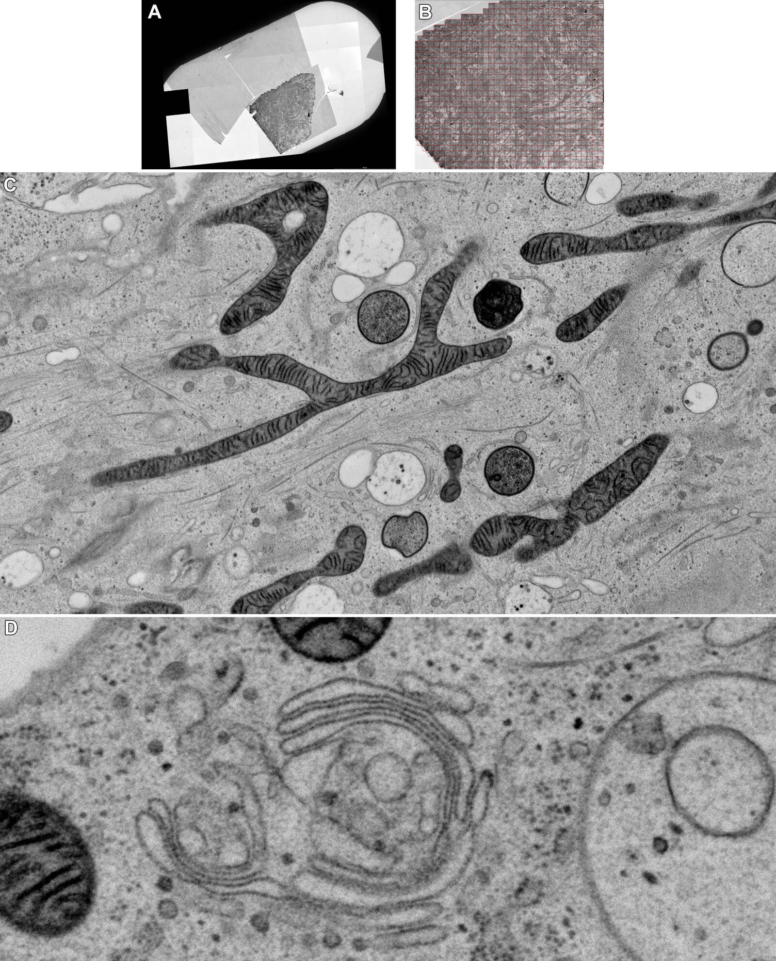
This technique, whether light or electrical stimulation, captures snapshots of particular events from multiple samples of the same specimen. It is, therefore, imperative to collect a large dataset. With recent advances in automated TEM (transmission electron microscopy), ultrathin sections can now be imaged overnight. Multiple images from a sample can be acquired automatically by shifting the compustage. All acquired images can subsequently be aligned and stitched to create one image with high-resolution data. The images shown here were acquired overnight using a Thermo Fisher Talos TEM operated at 120 kV. Thermofisher MAPS was used for automated acquisition of high resolution images from large areas.
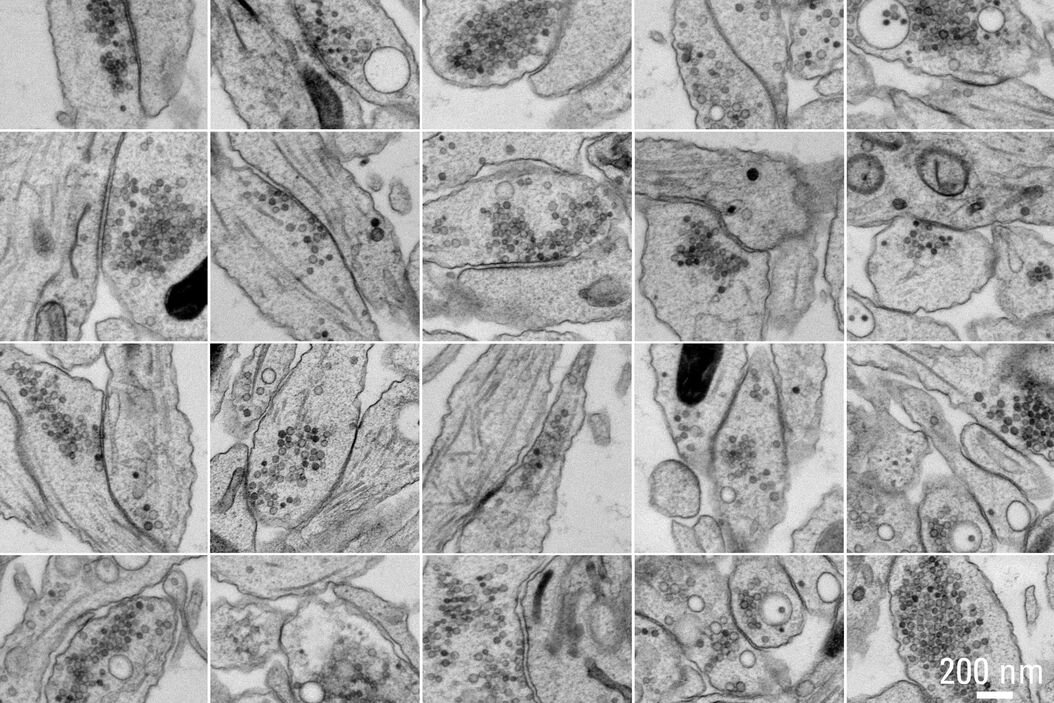
Figure 5A and 5B show stitched overview images of a control sample (no electrical stimulation). Figure 5C shows the processed sample in more detail. No cryoprotectant was used to freeze the sample. Both microtubules and actin filaments can be clearly resolved. The quality of freezing is uniform across the entire sample. After overnight acquisition, the entire dataset can be further analyzed off-line using the Thermofisher MAPS software. The images of the regions of interest can be aligned and stitched if necessary. The 25 hippocampal synapse images shown in Figure 6 were selected in about 10 minutes during a review of the data.

of these 25 synapses took approximately 10 minutes. Specimen and image courtesy of G. Bosshard and S. Tyagarajan, Institute of Pharmacology and Toxicology, and A. Kaech,
Center for Microscopy and Image Analysis, University of Zurich, Switzerland.
Read more
Detailed information on preparation and handling can be found in the
publication:
Li, S., Raychaudhuri, S., Watanabe, S. Flash-and-Freeze: A Novel Technique to Capture Membrane Dynamics with Electron Microscopy. J. Vis. Exp. (123), e55664, DOI: 10.3791/55664 (2017).
External
Related Articles
-

History, Developments and Trends of Microscopy in Cancer Research
Cancer is a global disease, with 18 million new cases diagnosed and 10 million cancer-related deaths…
Mar 16, 2026Read article -

Integrated Serial Sectioning and Cryo-EM Workflows for 3D Biological Imaging
This on-demand webinar explores how integrated tools can support electron microscopy workflows from…
Jul 22, 2025Read article -

Revealing Sodium Battery Degradation via Cryo-EM and CryoFIB
Explore how cryogenic electron microscopy and focused ion beam techniques uncover the intrinsic…
Jul 22, 2025Read article
