
For very fast kinetics the FlyMode can be applied. In this mode, reading out the signal during the x-fly back of the scanner provides a time resolution between lines, instead of frames, for the FRAP experiment. Depending on the necessary photobleaching power, you may choose ROI photobleach or ROI with Zoom In photobleach combined with one or multiple photobleach steps. The free y-format will reduce scanning time during photobleaching if multiple photobleach intervals are needed.
The FRAP wizard has improved functionality. With the introduction of the TCS SP8 microscope, the FRAP wizard offers you additional features:
- z-stacking;
- loop between photobleach and post-photobleach 1;
- sequential scan between lines; and
- Zoom In (“FRAP Zoomer”) for photobleaching in RS mode.
FRAP – step by step
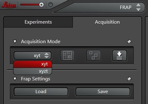
Choose the FRAP-Wizard
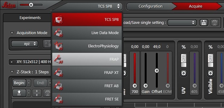
First, choose the FRAP-wizard option under “TCS SP8” at the top of the User Interface (UI) [Figure 1].
At the top of the wizard interface, the working steps are displayed as buttons: “Overview”, “Set Up”, “Bleach”, “Time course”, “Evaluation” (Figure 2).
The overview gives a description of the wizard and explains what to do in each step.
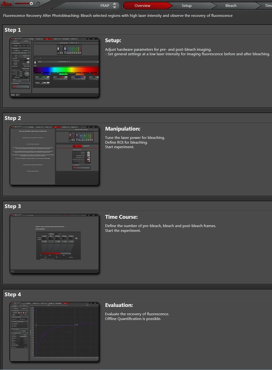
Step 1: Setup – Setting parameters for pre- and post-bleach
Imaging
First, the FRAP routine with Zoom In is described:
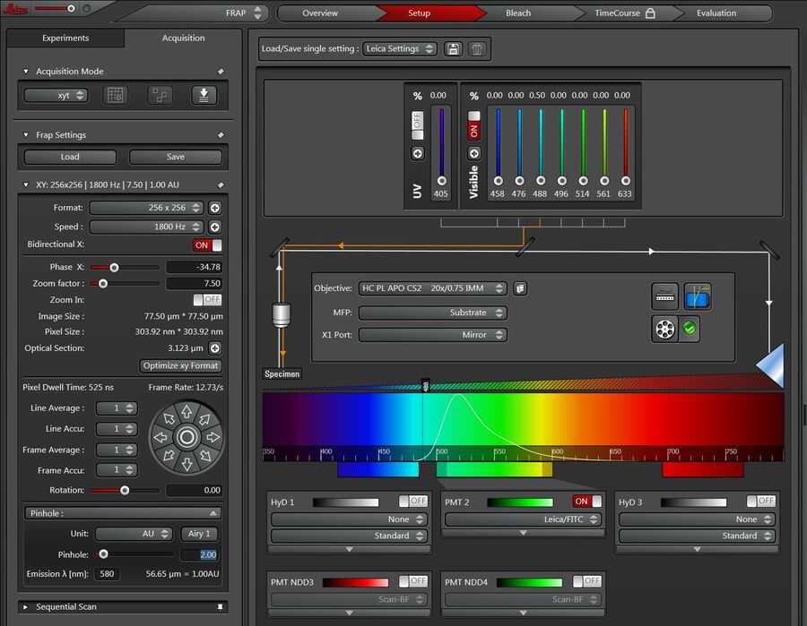
Click on the Setup button (see below in Figure 3) to adjust the hardware parameters for pre- and post-photobleach imaging.
Please Note:
On TCS SP8 systems equipped with Hybrid Detectors (HyDs), it is recommended to use a PMT as the detector of choice for the FRAP experiment. During the photobleaching sequence, typically high intensity levels are reached inside the Region Of Interest (ROI) which may cause the HyD detectors to switch off to protect them from photon-overload. As the detector has then to be switched on actively afterwards, the post-photobleach sequence will be lost and no quantification can be done.
Scan Mode
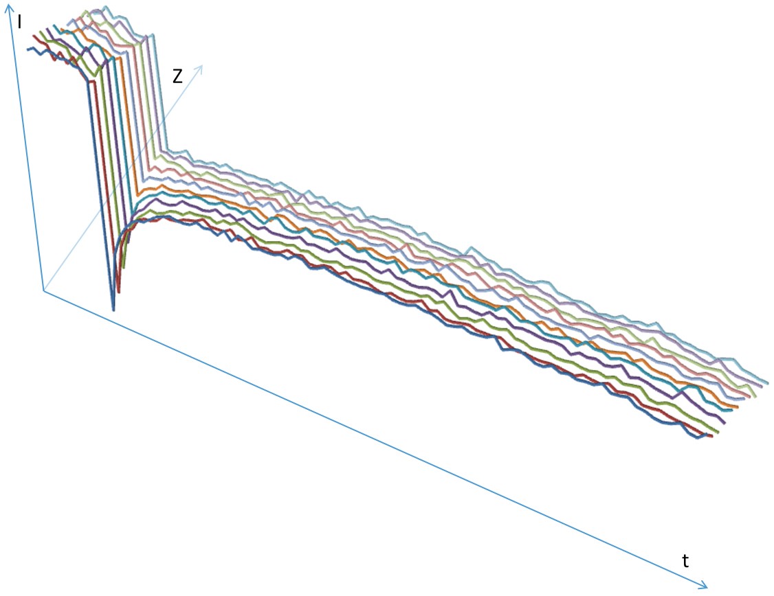
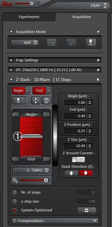
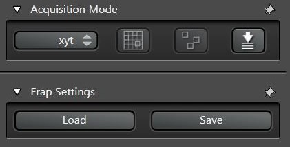
If a 3D stack should be analyzed in more detail, one can change the scan mode from xyt to xyzt (Figure 4) and analyze a whole z-stack over time. Pre- and post-bleach series are then scanned in xyzt mode and photobleaching of one plane within the stack can be defined.
Any plane within the stack can be defined for photobleaching. The position of the actual z-plane (Figure 5; ①) will be saved automatically and is displayed at the bottom of the UI. The photobleach pulse will only be executed in this plane. There will be no acquisition of a z-stack in the photobleach step.
Acquisition speed
Depending on the expected mobility of the molecules, the appropriate acquisition speed can be adjusted. Thus, for freely diffusing molecules a bidirectional scan speed of 1800 Hz line frequency should be used. In combination with an image format of 256 x 256 pixels, one can record an image every 79 ms.
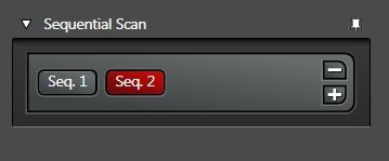
Sequential Scan
Choose sequential scan (Figure 6) to avoid crosstalk in the case of a multiple channel setup. This scan mode is also useful for photoconversion, i.e., experiments with photoswitchable proteins like KAEDE or DENDRA2.
Light Dose
To allow the highest dynamic range between monitoring and photobleaching, adjust the Argon laser power to be within the range of 80-100% (Figure 7) in the configuration/laser menu.
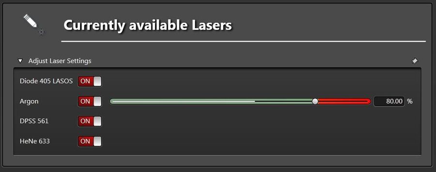
For imaging, set the AOTF (acousto-optical tunable filter) values to a low percentage.
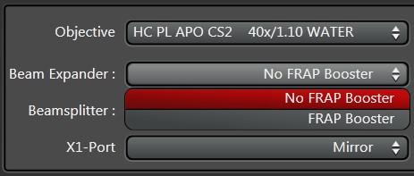
FRAP Booster
In case the amount of excitation light is not sufficient (e.g., during fast acquisition with resonant scanning) the option FRAP Booster (Figure 8) is recommended, assuming that the system is already configured with it. Once activated, the FRAP Booster option remains active for the whole experiment.
If this option is active, the beam expander is retracted from the beam path. As a result, the back aperture of the objective is no longer completely filled with light (see Figure 9A). The amount of light entering the objective is the same, but concentrated to a spot in the center, The light intensity is about 2 to 5 times greater, depending on the objective (see Figure 9B). In fact, the specimen can be illuminated with multiple amounts of light intensity (more concentrated versus less concentrated light) using the FRAP-Booster option.
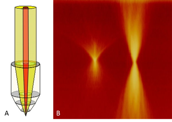
(B) Beampark experiment with a fluorescent slide. Much more light was applied to the sample using the FRAP Booster option. After beam-park, a xzy scan was done and processed to a maximum projection. Left: without FRAP Booster. Right: with FRAP Booster.
Pinhole Size
You may set the pinhole sizes to 2 airy units or more if you work with thin cell layers. Opening of the pinhole improves the signal-to-noise ratio and you will collect more information about kinetics deeper within the specimen.
Please note:
Set the intensity below saturation, but slightly above zero as a zero setting can interfere with data analysis. An appropriate lookup table (glow over/glow under) can help to adjust the gain/offset. Make sure to use the same gain settings for all experiments. For reproducibility, it is recommended to save (Figure 10) all settings from the Setup -, Bleach - and Time Course – Tabs either now or in the very last step. Then all hardware settings, including the ROI shape and position, will be stored.
Step 2: Bleach – Define parameters for photobleaching
Click on the Bleach - button (Figure 11) to set the parameters for photobleaching. On the left side you see a description of all options.
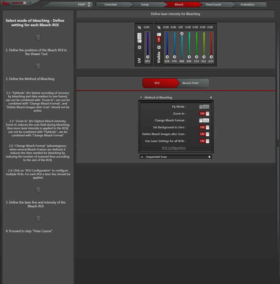
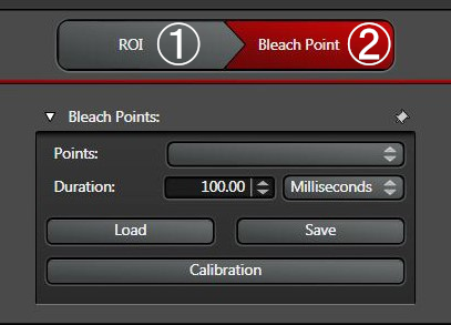
First, choose whether ROI ① or point bleach ② (Figure 12) should be applied.
You can choose any of the following options (Figure 13):
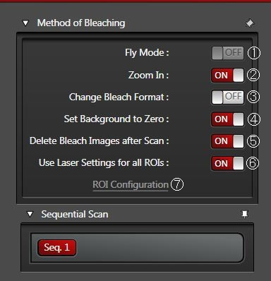
Fly Mode ①
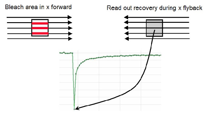
Allows faster time resolution for the whole FRAP series. Instead of frame-wise time resolution, line-wise time resolution can be achieved. You may reduce the time resolution down to 0.35 ms, because the recovery measurement is already done between lines instead of between frames. This fact means the recovery measurement starts as close as possible to the zero time (t0).
The FlyMode combines both the photobleach scan and first image scan after photobleaching (Figure 14). Photobleaching is performed during the forward motion using ROI scan features together with high laser power. During the flyback, the laser intensity is set to imaging values (AOTF switching works within microseconds). Thus, the first image is acquired simultaneously with the photobleaching frame. Consequently, the delay time between bleaching and data acquisition is less than half the time needed to scan a single line.
Zoom In ②
For most photobleaching applications, we recommend the Zoom In option. The scan field during photobleaching is then minimized and more light is applied to the ROI.
With the TCS SP8 system, a zoom-In is also possible with the resonant scanner.
Change Bleach Format ③
In accordance with the size of the defined ROIs, the number of scanned lines is reduced during photobleaching (strip scan). You may use this option to speed up the photobleaching when multiple intervals, e.g. 10 or more, are needed. This option can be combined with Zoom In.
Set Background to Zero ④
This option is recommended when Zoom In or FlyMode is active.
Zoom In:
Normally, the area outside of a ROI will be exposed to the background intensity. This background intensity can lead to photobleaching if the image is zoomed in. Using “Set background to zero” the area outside the exposed ROI will get no light.
FlyMode:
When the FlyMode is active, you have a forward channel and a fly back channel (see above). Using “Set background to zero” the forward channel will see no light during prebleach and postbleach. Only during the photobleach step will the forward (left) channel get light inside the ROI.
Delete Bleach Images after Scan ⑤
Usually the photobleached ROI is very bright and in many experiments Zoom In for photobleaching is used, but it hampers meaningful quantification. The same is valid for the option “Change Bleach Format”. For these cases, the option “Delete Bleach Images after Scan” avoids accumulation of waste data.
Use Laser Settings for all ROIs ⑥
When several ROIs should be exposed with the same laser lines, one can choose this option. Now draw the ROI for bleaching and define the AOTF value(s) to tune the laser power for bleaching.
Photo bleaching with several laser lines and ROIs
Click on ROI Configuration ⑦ when individual laser lines should be active for several ROIs. In advance, you have to uncheck “Use laser settings for all ROIs”.
Preconditions for effective photobleaching in resonant scanning mode
If very fast scan modes are needed (e.g., measurement of diffusion in aqueous media) you may scan bidirectionally in 512 x 128 format which results in a very short time per frame, i.e. 12 ms. Here it is recommended to apply multiple photobleach frames, e.g., three or four, to apply sufficient light for photobleaching.
To compensate for too little light due to a short illumination time, you may use:
- Zoom In during photobleaching (with the TCS SP8 system, Zoom In is available for the resonant scanner as well) [FRAP Zoomer].
- the FRAP Booster option within Set Up.
Photoactivation
You can use the FRAP wizard for photoactivation (e.g., when using PA-GFP) as well. Open the UV-shutter and then use in the photobleach step the 405 laser line instead of the 488 laser line.
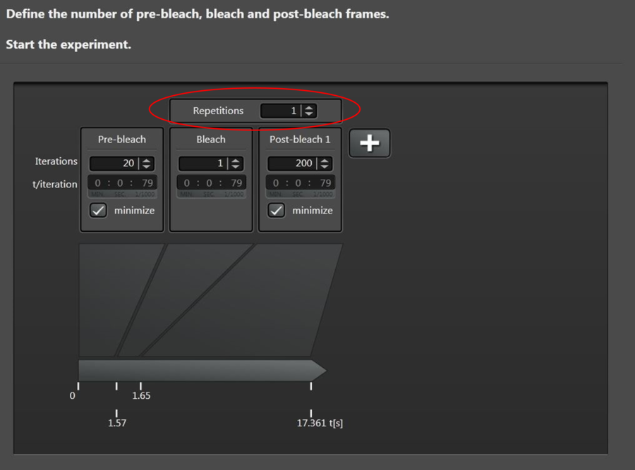
Step 3: Time Course – Define number of prebleach, bleach and postbleach intervals
Next, choose Time Course (Figure 15) to define number of prebleach, bleach and postbleach intervals. A typical experiment with 1800 Hz scan speed (bidirectional scan) and 256 x 256 format can be defined as follows:
You may add, as well, additional timescales by clicking “+”. If needed, the experiment can be stopped in the middle of a run, e.g., during postbleach. The user will then be guided to the evaluation step. This feature is particularly useful if the total time for full recovery is not known, because it allows the user to end the experiment during postbleach as soon as full recovery (i.e., no more increase in intensity) is reached. In other words, there is no need to wait until the predicted number of frames has been acquired.
| # frames | minimized time frame | time per frame [ms] |
Prebleach | 10 | yes | 79 |
Bleach | 1 | yes | 79 |
Postbleach 1 | 100 | yes | 79 |
Postbleach 2 | 10 | no | 1000 |
Postbleach 3 | 10 | no | 5000 |
Table 1: Total frame and frame rate parameters of the prebleach, bleach, and postbleach steps.
Acquisition speed
The acquisition speed should be adjusted to resolve the dynamic range of the recovery with good temporal resolution. Thus, ideally acquire at least 10 data points during the time required for half of the recovery.
FRAP with Loop
To do FLIP experiments, you can set the number of repetitions ① (Figure 15) between the bleach and first postbleach steps.
Duration of the FRAP experiment
Initial experiments should be conducted until no noticeable further increase in fluorescence intensity is detected. If you want your ROIs & Time Course included in your saved settings, you can do this in Step 1 or the last step. Click Run Experiment to start the experiment. It runs automatically and then leads to the evaluation step.
Please note:
If you do experiments with fluorescent proteins, usage of postbleach sequences with different timescales may lead to an intensity decrease during the timescale transitions. Changing the imaging frequency during the experiment can alter the fraction of fluorescent proteins driven into dark states (refer to reference 16 below). Another strategy is to define 40 or 50 prebleach intervals to achieve a steady state intensity after an initial intensity decrease within the first 10 to 20 intervals of the prebleach series.
Step 4: Evaluation
Now the recovery chart is displayed (Figure 16). The chart shows all intensity values averaged over the ROIs for all frames. This chart can be exported to Excel via a right click with the mouse.
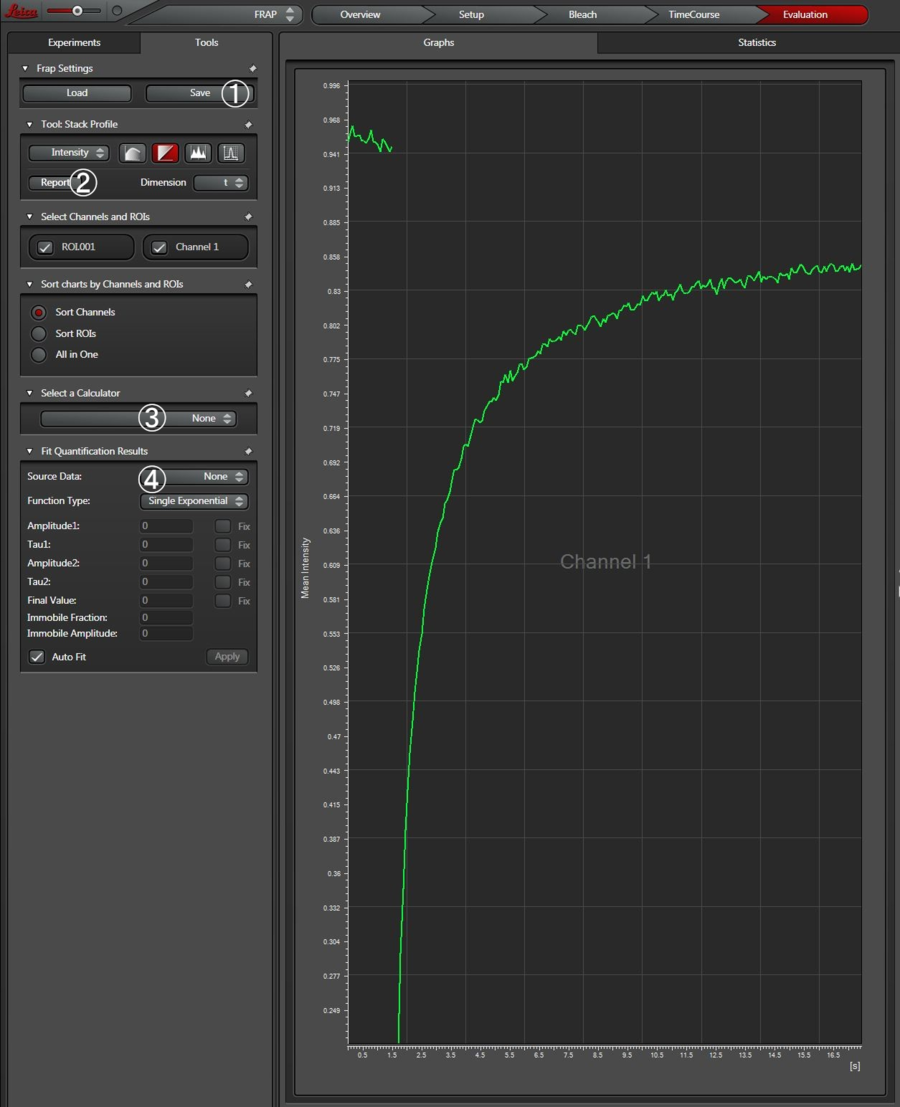
- Experimental conditions and procedures can be saved;
- Report generates a data sheet in xml format;
- Background can be subtracted;
- Fitting can be applied to the data;
Download pdf
Confocal Application Letter - FRAP with TCS SP8 (pdf, 2MB)
 in 14 x 18 tiles. Lifetime gives an additional contrast that allows to differentiate different structures in histological stainings.")